Category: Uncategorized

This is a review of the journal article “Motivational Profiling of League of Legends Players” by Brühlmann et al., 2020 [1]. 

Overview

The authors use an Organismic Integration Theory (OIT) based questionnaire called the User Motivation Inventory (UMI)[2], which is designed to measure player motivational regulations. After gathering 750 participants from the League of Legends subreddit (predominantly 17-25 year old males) they used the responses to this questionnaire to identify motivational profiles using Latent Profile Analysis (LPA)[3]. Responses to several other Self-Determination Theory (SDT), wellness, and experience based questionnaires, as well as in-game behaviour metrics, were also collected. These were aggregated and compared between the four different identified motivational profiles.

The authors find statistically significant differences in play experience based measures (how the player perceives the play experience and how it affects them) between the four identified profiles. They also find some statistically significant differences in play behaviour (what the players actually do when playing the game) between the four profiles.

Research Problem & Gap

Motivation, and SDT in particular, is a key research area within games research [5], but literature investigating how the motivational regulations of players affects the play experience and in-game behaviours is lacking.

There is also limited empirical work investigating how differences in motivational regulation affects psychological needs satisfaction. In other words if a player feels amotivated, extrinsically motivated, or intrinsically motivated, how does this impact the players’ psychological needs for competence, autonomy and relatedness when interacting with videogames? This paper aims to address these questions.

Contribution(s)

1. The authors utilise a method to cluster responses to the User Motivation Inventory (UMI) questionnaire to identify four motivational regulation profiles of League of Legends players via a process called Latent Profile Analysis (LPA). 
2. These profiles are correlated with several other questionnaire responses designed to measure interest/enjoyment and pressure/tension, needs satisfaction, wellbeing, positive and negative associations, goal achievement and harmonious and obsessive passion. Doing so the authors show statistically significant differences in experience between players of different motivational profiles.
3. The profiles are also used to compare aggregated in-game behaviour metrics between profiles, demonstrating some statistically significant differences in game playing behaviour (albeit less significant relative to the reported experience differences).
4. This empirically validates that motivational regulations are related to the play experience and in-game behaviours of players of MOBA games.

Methods

Several SDT, wellbeing, and other psychological measures (questionnaires) are utilised where response are given using mostly answered using 5 or 7-point likert scales:

• User Motivation Inventory (UMI): a questionnaire based on the Organismic Integration Theory subtheory of SDT. This measures 6 factors including: amotivation, external regulation, introjected regulation, identified regulation, integrated regulation and intrinsic motivation.
• Player Experience Needs Satisfaction (PENS)[6]: a post-hoc SDT based questionnaire measuring needs satisfaction for competence, autonomy and relatedness.
• Vitality[7]: a measure intended to capture impacts on wellbeing (positive or negative).
• Intrinsic Motivation Inventory (IMI)[8]: the authors specifically adopt the interest-enjoyment and pressure-tension dimensions of the IMI. Authors hypothesise that these are experienced regularly by MOBA players.
• PANAS[9]: a measure intended to capture positive and negative affect. Authors hypothesise that these are experienced regularly by MOBA players.
• Achievement Goals[10]: measures a player’s achievement goals orientation (one of: mastery approach, mastery avoidance, performance approach and performance avoidance).
• Harmonious and Obessive Passion (HOP)[11]: a measure to identify autonomous and self-determined internalisation which does not interfere with other areas of life (harmonious), as well as identify non-self-determined internalisation due to external or internal pressure which may interfere with other areas of life (obsessive).

In-game behaviour metrics are also collected via the League of Legends API using participants’ provided summoner names (usernames). These aggregated metrics included time played, level, total matches, kills, assists, win rate, etc.

Latent Profile Analysis (LPA) is conducted on the responses to the UMI questions in order to identify four different motivational regulation profiles of the LoL players. Bayesian Information Criterion (BIC), Integrated Complete-data Likelihood (ICL) and Bootstrap Likelihood Ratio Test (BCLR), as well as authors’ own understanding of the profiles’ theoretical conformity were used to identify the appropriate number of profiles from the data.

The reason for conducting this Latent Profile Analysis was to produce profile labels which enable multi-dimensional analyses. For example, consider if one participant answered the intrinsic motivation (IMO) questions of the UMI very highly, but also answered the amotivation (AMO) questions highly. This participant may be very dissimilar to another participant who responds highly for IMO but low for AMO. The first participant may belong to the Amotivated profile, whereas the second would almost certainly belong to the Intrinsic profile. If we only considered high respondents for IMO as intrinsically motivated players, we would consider these two players the same. Hence clustering methods like LPA are necessary to perform more nuanced, multi-dimensional, and person-centric analyses. People are not one-dimensional, so our analyses should not be either!

The four profiles (and their distribution of values on each latent variable of the UMI) are shown above in Figure 3. Notice how Amotivated and External are similar, and Intrinsic and Autonomous are also similar. We will discuss these similarities later.

Results

Behavioural Game Metrics

The authors conducted a correlation analysis between the profiles and aggregated in-game metrics. These tell us how players who fit into each profile behave in the game on average.

Some interesting results pop up. First is that there aren’t many significant differences in the behaviour of the four different profiles. The main significant behavioural differences are: amotivated and autonomous players have higher mean winrate in unranked games, autonomous players have higher mean KDA in ranked games, and autonomous players have higher mean assists in unranked games. The remaining differences are not statistically significant.

Combined with the similarity of the profiles as per the UMI factors (Figure 2 above), the question arises as to why these profiles seem so similar. We’ll tackle this question shortly.

Player Experience

The authors also aggregated the results for responses to the other measures (questionnaire questions) by profile to see what the difference in player experience was between each profile. These tell us various things such as the extent to which the players experienced enjoyment, tension, feelings of positive/negative well being,  psychological needs satisfaction and so on. The results are more interesting and are summarised below in Figure 5.

Describing this plot from left to right. All profiles reported high enjoyment, with the Intrinsic profile reporting highest levels of enjoyment. This is consistent with Organismic Integration Theory (see Figure 1), which posits that more integrated external regulations have more significant positive effects on wellbeing, engagement and enjoyment of an activity. Intrinsic motivation is believed to be the superior form of motivational regulation producing the highest levels of engagement, wellbeing and enjoyment.

Externally motivated players reported highest levels of tension. This may be due to their motivational regulation focussing on external outcomes, such as feeling pressure to perform well in the game to please their teammates, or to realise some internalised expectation of their own performance. 

Intrinsically motivated players reported the highest levels of needs satisfaction for autonomy, which is also consistent with Organismic Integration Theory. There were not large differences in needs satisfaction for competence among the profiles, but Intrinsic and Autonomous reported slightly higher levels. For relatedness, the Amotivated profile reported significantly lower levels of needs satisfaction. This might indicate that Amotivated players do not feel a sense of connection or community with their fellow players whilst playing the game, and possibly avoid others whilst playing. This is consistent with their behavioural metrics: Amotivated players provide the lowest numbers of assists in both ranked and unranked, the highest number of kills in ranked mode, and the highest number of deaths in ranked and unranked. This suggests a maverick/solo playstyle for Amotivated players.

In terms of goal achievement, a standout result is that Intrinsically motivated players report the lowest levels of mastery and performance avoidance. This suggests that Intrinsically motivated players are not concerned with losing previously acquired knowledge or skills and are not concerned with performing worse than their peers or some normative standard. These goals are significantly higher for externally regulated players, from which we can infer they play due to an external or internalised pressure to perform highly and not lose their skill.

This result is supported by the significantly higher responses for obsessive passion for External regulated players. While not a high average response, it suggests their play habits might be more likely to interfere with other aspects of their lives in an unhealthy way. In contrast, intrinsically motivated players report the highest levels of harmonious passion, which is defined as “the autonomous and self-determined internalization of an activity into one’s identity (Vallerand et al., 2003), whereby the activity is aligned with different areas of a person’s life”. 

The responses for Vitality support this finding further, where the Intrinsic profile reports the highest levels of Vitality and External reports somewhat lower levels of vitality. Vitality in this instance is defined as “positive feelings of aliveness and energy … hypothesized to reflect organismic well-being.”
However, the Amotivated profile reports the lowest levels of vitality, suggesting that disengagement and lack of understanding of why one plays LoL is somewhat detrimental to wellbeing.

Summary and Critical Reflection

In this paper the authors have demonstrated that different types of motivational regulation can relate to the player experience and in-game behaviour. The authors highlighted the distinction between motivational regulations (OIT) and psychological needs satisfaction (SDT), and how these two interact during gameplay. Their empirical analysis is extended to include measures of wellbeing, demonstrating that the different types of motivational regulation also impact players’ experience differently, with intrinsic motivation and more integrated forms of external regulation being the most desirable for player wellbeing.

The side-by-side comparisons of so many psychological measures in one study of video game players is extremely interesting and applicable to industry.

However, the sampling method may have biased the results towards players of a specific demographic (17-25 year old males) who are probably all highly engaged (interacting outside of the game on the subreddit is a strong indicator of overall engagement). This might explain why the four identified motivational profiles are very similar, in terms of the underlying UMI measure, additional measures, and in-game behaviours. Casting the net wider to find participants with varied levels of engagement might yield different results with more significant differences between the types of players.
In addition to the above, this use of gameplay behaviour metrics aggregated over the lifetime of the player assumes that a player’s motivational profile is static over the course of their interactions with a game. This is a big assumption. It assumes that motivational regulations are traits rather than states of the player. In other words: is it possible for a player to change from one motivational type to another over the lifetime of their engagement with a game, or even during the same play session? Organismic Integration Theory asserts that this is the case. If it is true, then comparing lifetime aggregated behavioural metrics between the profiles is less likely to reveal significant differences in behaviour.

References

[1] F. Brühlmann, P. Baumgartner, G. Wallner, S. Kriglstein, and E. D. Mekler, ‘Motivational Profiling of League of Legends Players’, Front. Psychol., vol. 11, 2020, Accessed: May 12, 2023. [Online]. Available: https://www.frontiersin.org/articles/10.3389/fpsyg.2020.01307

[2] F. Brühlmann, B. Vollenwyder, K. Opwis, and E. Mekler, ‘Measuring the “Why” of Interaction: Development and Validation of the User Motivation Inventory (UMI)’, Apr. 2018. doi: 10.1145/3173574.3173680.

[3] D. Spurk, A. Hirschi, M. Wang, D. Valero, and S. Kauffeld, ‘Latent profile analysis: A review and “how to” guide of its application within vocational behavior research’, J. Vocat. Behav., vol. 120, p. 103445, Aug. 2020, doi: 10.1016/j.jvb.2020.103445.

[4] Handbook of self-determination research. in Handbook of self-determination research. Rochester, NY, US: University of Rochester Press, 2002, pp. x, 470.

[5] A. Tyack and E. D. Mekler, ‘Self-Determination Theory in HCI Games Research: Current Uses and Open Questions’, in Proceedings of the 2020 CHI Conference on Human Factors in Computing Systems, Honolulu HI USA: ACM, Apr. 2020, pp. 1–22. doi: 10.1145/3313831.3376723.

[6] R. M. Ryan, C. S. Rigby, and A. Przybylski, ‘The Motivational Pull of Video Games: A Self-Determination Theory Approach’, Motiv. Emot., vol. 30, no. 4, pp. 344–360, Dec. 2006, doi: 10.1007/s11031-006-9051-8.

[7] R. M. Ryan and C. Frederick, ‘On Energy, Personality, and Health: Subjective Vitality as a Dynamic Reflection of Well-Being’, J. Pers., vol. 65, no. 3, pp. 529–565, 1997, doi: 10.1111/j.1467-6494.1997.tb00326.x.

[8] E. McAuley, T. Duncan, and V. V. Tammen, ‘Psychometric Properties of the Intrinsic Motivation Inventory in a Competitive Sport Setting: A Confirmatory Factor Analysis’, Res. Q. Exerc. Sport, vol. 60, no. 1, pp. 48–58, Mar. 1989, doi: 10.1080/02701367.1989.10607413.

[9] D. Watson, L. A. Clark, and A. Tellegen, ‘Development and validation of brief measures of positive and negative affect: the PANAS scales’, J. Pers. Soc. Psychol., vol. 54, no. 6, pp. 1063–1070, Jun. 1988, doi: 10.1037//0022-3514.54.6.1063.

[10] A. J. Elliot and H. A. McGregor, ‘A 2 X 2 achievement goal framework’, J. Pers. Soc. Psychol., vol. 80, no. 3, pp. 501–519, Mar. 2001, doi: 10.1037/0022-3514.80.3.501.

[11] R. J. Vallerand et al., ‘Les passions de l’âme: On obsessive and harmonious passion.’, J. Pers. Soc. Psychol., vol. 85, no. 4, pp. 756–767, 2003, doi: 10.1037/0022-3514.85.4.756.

In the last post we discussed the problem of acting optimally in an episodic environment by estimating the value of a state. Monte Carlo Tree Search (MCTS) naturally fits the problem by incorporating intelligent exploration into decision-time multi-step planning. Give that post a read if you haven’t checked it out yet, but it isn’t necessary to understand today’s post. It might also be beneficial to get some intuition on UCB action selection.

Today we’re going to dig into ‘vanilla’ MCTS, the same algorithm used in state of the art game-playing agents like AlphaZero. When we’re done you’ll understand how and why this works so well for general game playing (especially in board games like Chess and Go).

Accompanying code snippets are included in the post to help explain the ideas. You can also follow along and run the code in this colab notebook. A python implementation of Connect4 is included in the notebook so you can play against the finished MCTS algorithm 😄 🔴🔵🔴🔴

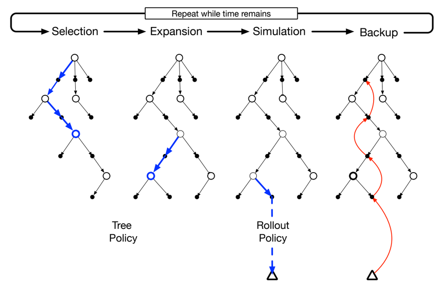
The Four Steps in MCTS:

MCTS builds up estimates for the values of each possible state and action by planning ahead. In order to do this it must have a perfect model of the environment. In other words it must know exactly where it ends up after taking each action – without actually having to take that action. This is a downside to MCTS, since it can’t work without this model.

Anyway, assuming we have this perfect model we can simulate taking actions and choose the best ones based on the outcomes of simulated games. Doing so repeatedly we can build up a game tree of actions and states the algorithm has explored 🌳. Here are the four steps MCTS repeats to do this:

1. Selection
2. Expansion
3. Rollouts/Simulation
4. Backup of results

1. Selection:

MCTS starts by selecting the best node in the tree so far according to the UCB formula. This formula estimates the value (and uncertainty in that value) of each state in the tree. This form of MCTS is actually called “upper-confidence bound applied to trees” (UCT). Furthermore, UCT is just an extension of UCB action selection from multi-armed bandit problems, but applied to multi-step decision making instead. Here’s the UCB formula adapted to tree search (with explanation below):

\begin{aligned}
Score_i &= \bar{q}_i + U_i \\
&= \bar{q_i}+C \sqrt{\frac{2 \ln N}{n_i}}
\end{aligned}

To demonstrate; think about this from the perspective of a parent node with several child nodes to consider. The action selection score of each child node is made up of the current estimate and uncertainty. The value estimate of the i-th child node is the current mean value of that node (\bar{q_i}). The uncertainty part has a constant C, that scales the uncertainty (bigger means more exploration, smaller means less exploration). We’ll leave this C=1. In the square root, N is the number of visits to the parent, and n_i are the number of times the child node i was chosen when passing through the parent N.

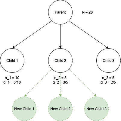
As an example, check the diagram below:

If we are in the parent node deciding which child node to explore, we apply the above UCB formula to each of the children and choose the one with the highest score. For instance evaluating child 1 and child 2:

\begin{aligned}
Score_1 &= \frac{5}{10} + \sqrt{\frac{{2\ln20}}{10}} = 1.274 \\
Score_2 &= \frac{3}{5} + \sqrt{\frac{{2\ln20}}{5}} = 1.694 \\
\end{aligned}

According to this score the action selection will decide to further explore child 2. This is because we have explored Child 2 only 5 times, but exploring that child won 3 out of the 5 simulated games! This is a high win rate. We are also less certain about this result because the number of times explored is low (5). So the UCB action selection correctly pushes the algorithm to further explore this promising node 🧭.

Important side notes !!!

1. When selecting from child nodes: if two children have an equal score, they must be selected from randomly. Any other tie-breaking method is not guaranteed to converge to an optimal policy.
2. Additionally if a child node has not been explored at all (no visits) we automatically set it’s Q+U value to be +infinity (to guarantee exploring any unexplored children when visiting a parent node).
3. Actually just about any bandit action selection algorithm could work in place of UCB. \epsilon-greedy for example.

Here’s the first part of the code in python, wrapped in a TurnBasedUCTNode class. We start in tree_policy():

class TurnBasedUCTNode():
  def __init__(self, 
               env, 
               player_1_state,
               player_2_state,
               player_turn,
               action=None,
               reward=None,
               parent=None,
               id_in_parent=None):

    self.env = env
    self.player_1_state = player_1_state # 2d np array
    self.player_2_state = player_2_state # 2d np array
    self.player_turn = player_turn
    
    self.action = action # which action was chosen previously Q(s,a)
    self.parent = parent # parent node

    # self.action != id_in_parent e.g. action may be 6, but id_in_parent may be 0
    self.id_in_parent = id_in_parent # index of this child in parent's list of children

    self.is_expanded = False
    self.children = [] # list of child nodes
    self.child_visit_count = None  # need to expand before we know size of this list
    self.child_q_sum = None  # need to expand before we know size of this list
    self.reward = reward

  def child_q_estimates(self):
    return self.child_q_sum/(self.child_visit_count+1)
  
  def child_ucb1_estimates(self):
    # handle case where we are at root with no parent
    if self.parent is None:
      my_visits = np.sum(self.child_visit_count)
    else:
      my_visits = self.number_visits

    U = np.sqrt(2.0*np.log(my_visits)/(self.child_visit_count+1))
    return U * EXPLORATION_CONSTANT

    
  def select_best_child(self, max_value=1e6):
    # Get Q + U for each child, return max, break ties randomly

    if not self.is_expanded:
      return self
    
    q_u = self.child_q_estimates() + self.child_ucb1_estimates()
    q_u[self.child_visit_count==0.0] = max_value

    max_choices = np.flatnonzero(q_u == np.max(q_u))

    if len(max_choices) == 1:
      return max_choices[0]

    random_choice = rando._randbelow(len(max_choices))
    best_child_index = max_choices[random_choice]

    return best_child_index

  def tree_policy(self):
    current = self

    node_visits = 0
    while current.is_expanded:
      node_visits += 1
      best_child_index = current.select_best_child()
      current = current.children[best_child_index]

    return current, node_visits # a not expanded leaf node

2. Expansion:

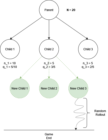
This part is pretty easy to understand. Once selection reaches a node that has no children, we need to create those children. So we are expanding the tree. We do this by asking our simulated environment (perfect world model) which actions we can take given the state we are in. Then we take each of these actions in turn in our simulated environment and store the resulting states as new child nodes. Once this is done, we select one of these at random for the rollout/simulation stage.

The code for the expansion step is below, it is a method of the TurnBasedUCTNode class:

def expand(self):

    if self.reward is not None:
      return self

    possible_actions = self.env.get_legal_actions(self.player_1_state, 
                                                  self.player_2_state)

    # perform action filtering in env.legal_actions to get legal actions
    action_num = len(possible_actions)

    if action_num == 0:
      return self

    next_player_turn = -1 if self.player_turn == 1 else 1 # flip player turn

    self.child_visit_count = np.zeros(action_num, dtype=np.uint32)
    self.child_q_sum = np.zeros(action_num, dtype=np.int32)

    # loop thru legal actions and simulate stepping each one
    i = 0
    for action in possible_actions:
      p1_state, p2_state, reward = self.env.step(action,
                                                  self.player_turn, 
                                                  self.player_1_state.copy(), 
                                                  self.player_2_state.copy())
      child = TurnBasedUCTNode(self.env, 
                                p1_state, 
                                p2_state, 
                                player_turn=next_player_turn, 
                                action=action, 
                                reward=reward, 
                                parent=self, 
                                id_in_parent=i)

      self.children.append(child)
      i+=1 # increment the index used for id_in_parent

    self.is_expanded = True

    # return a random child node for rollouts
    random_child = self.children[rando._randbelow(len(self.children))]                                              

    return random_child

3. Rollout / Simulation:

This part is pretty fun, and is at the heart of why MCTS works. It took me a while to get my head around this when I was first learning about MCTS. So I’ll spend some extra time on this section to map out the concepts and intuition.

You may have been wondering where the \bar{q_i} part came from in the UCB formula discussed earlier. It’s made up of two parts: the number of visits, and the sum of rewards. The number of visits makes sense, but where does the sum of rewards come from? It comes from the Monte Carlo rollouts 🧻.

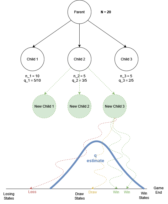
In this stage the algorithm simulates a full game (all the way to the end) by randomly selecting actions for each player until the simulated game ends. Once that happens, the environment tells us if the game ended in a win/loss/draw, which is the reward.

To clarify during rollouts we don’t need to create new nodes and copy state variables. Therefore the rollout stage is fast.

This still doesn’t really explain why rollouts work though. How does the result of a random game help us decide which actions to take?

A great way to think about this is as an extension of multi-armed bandit problems. In M.A.B.s we usually sample an action several times to build an estimate of its value. The same thinking applies here too. Hence, the more times we expand, reach a leaf node, and randomly rollout, the better the estimate of the value of each node/action.

To make this clearer: imagine if we sorted all of the possible end-game states from left to right, in order of lose, draw, win (see the diagram below). So a winning rollout will always land to the right, and a losing one to the left, and a draw is somewhere in the middle. In this visualisation we can imagine that good actions move us to the right, whereas bad actions move us to the left.

Consider that for any node we are building the probability density function of the rewards from the simulated games (-1, 0, +1). Therefore the q-estimate of a node is the mean of this p.d.f generated from rollouts that passed through this node. This allows us to determine if an action is good or bad! 😈

Code for the rollout method is shared below to neatly summarise:

def rollout(self):
    max_t = (self.env.board_height*self.env.board_width)
    # If this node is terminal state, backup reward immediately
    if self.reward is not None:
      self.backup(self.reward)

    reward = None

    temp_p1_state = self.player_1_state.copy()
    temp_p2_state = self.player_2_state.copy()
    rollout_turn = self.player_turn

    while i < max_t:
      # get legal actions from the environment
      legal_actions = self.env.get_legal_actions(temp_p1_state, temp_p2_state)

      # In this case, must be a draw.
      if not legal_actions:
        reward = 0
        break

      # choose random actions during rollouts
      action = legal_actions[rando._randbelow(len(legal_actions))]

      # don't need to copy states during rollout steps, just act on same state
      temp_p1_state, temp_p2_state, reward = self.env.step(action,
                                                            rollout_turn,
                                                            temp_p2_state, 
                                                            temp_p1_state)

      # reward signals end of game
      if reward is not None:
        # reward is -1 if the player turn is not same as rollout turn
        # in other words: this action led to eventual loss
        if rollout_turn != self.player_turn:
          reward = reward * -1
        break

      # flip player_turn on each loop
      rollout_turn = -1 if rollout_turn == 1 else 1

    self.backup(reward) # backup the reward

4. Backup:

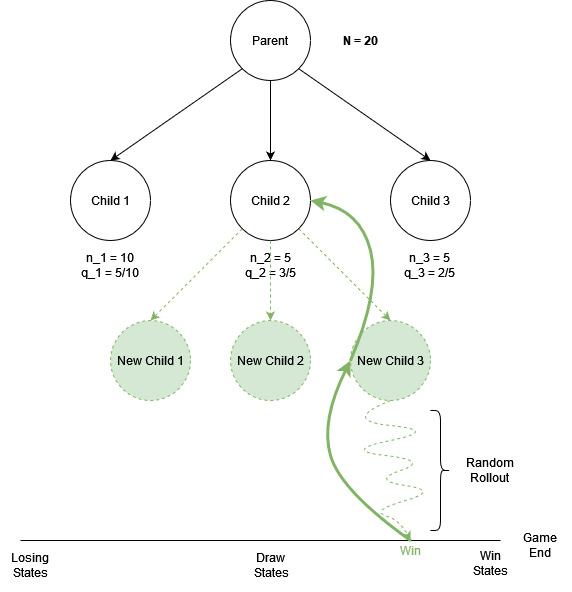
Once a rollout is complete we have to traverse the tree backwards and update the \bar{q_i} estimate of each node. This is done by incrementing its visit count and adding the reward from the rollout to its reward sum. Again, we need to backup so that each node is aware of the outcomes of games that ‘passed’ through it.

We first update the values in the leaf node, then move to the parent of that node and update those values, and so on. Until we reach the root node. At this point there is no parent, and we don’t need to update the values of the root node anyway.

Code for the backup method is provided below. Beware: we backup in a NegaMax fashion. Meaning we negate the value of the reward on each visit to subsequent parent nodes. Why? Because Connect4 is a two-player turn based game, so every second node is an opponent move. A win for us is a loss for the opponent. During the selection phase this allows MCTS to simulate the opponent picking the ‘best’ moves from their perspective during their turns! 🧠

 def backup(self, reward):
    current = self

    if reward is None:
      reward = 0.0

    # in case we reached root
    while current.parent is not None:
      current.number_visits += 1
      current.total_value += reward 
      current = current.parent
      reward = reward * -1 # Ensure correct sign when backing up rewards

Playing against MCTS in Connect 4:

Now it’s time to play against the AI we have created 🙂 You can do so by running the colab notebook, and interacting with the game at the very bottom of the notebook. 🔴🔵🔴🔴

1. Open the link.
2. At the top, click “Runtime”.
3. Press “Run All”
4. Scroll to the bottom and enter your moves in the text box (you are circles, see image below).

Adjusting the difficulty: The MCTS agent will take 5 seconds per turn. You can adjust the difficulty by giving the agent more or less time. Do this by passing adjusting the time_limit parameter in the uct_search function call.

for i in range(0, max_turns):

  # p1: looks ahead using MCTS
  root_node = TurnBasedUCTNode(env, p1_state, p2_state, player_turn=1)
  action = uct_search(root_node, time_limit=7.0)
  print(f"Chosen action: {action}")

Summary:

We’ve seen how the MCTS algorithm works step by step. In summary: first the algorithm repeatedly selects nodes using the UCB action selection formula until it reaches a leaf node. It then expands a leaf node to create new child leaf nodes. Next, randomly selecting a new child leaf, the algorithm simulates a random game all the way to the end. The result or reward from that simulated game is then backed up the tree by revisiting each parent node. Furthermore, MCTS goes through this process repeatedly until some terminal condition is reached (usually a time limit). 📝

MCTS is one of the few general game playing algorithms out there. It doesn’t have any game-specific logic hard coded into it. Meaning we could drop the same algorithm into a different game like Chess and it would still work. All it needs is a simulator environment.

However, it also has its flaws. One of these is the need for the simulator environment – MCTS cannot plan ahead without one. This limits its use to situations where we have a simulator.

Future Work:

A relatively simple problem we could solve is that on every turn we build a brand new tree, decide on an action, and then throw the tree away. This means we’re rebuilding a lot of the same parts of the tree over and over again! With this in mind we could re-use the tree rather than starting from scratch each turn.

Another problem we could address is with the game-theoretic convergence. This means that in immediate sudden-death situations the algorithm must simulate many times in order to converge on the game theoretic win/loss value. We can address this problem by implementing a MCTS-Solver (a topic I’ll cover in future). 🛣️

Thanks for reading! 🙂